Working with Time Series Data

This example shows how to load the included smartwatch inertial sensor dataset, and create time series data objects compatible with the seglearn pipeline.

Out:

DATA STATS - AGGREGATED
{'n_series': 140, 'n_classes': 7, 'n_TS_vars': 6, 'n_context_vars': 2, 'Total_Time': 4882.04, 'Series_Time_Mean': 34.87171428571428, 'Series_Time_Std': 8.757850351285423, 'Series_Time_Range': (18.94, 52.36)}

DATA STATS - BY CLASS
  Class_labels  n_series  Total_Time  Series_Time_Mean  Series_Time_Std  Series_Time_Min  Series_Time_Max
0          PEN        20      532.44            26.622         2.720845            21.28            31.10
1          ABD        20      798.10            39.905         8.055554            22.48            49.10
2          FEL        20      809.96            40.498         8.772099            22.30            50.84
3           IR        20      747.90            37.395         9.085212            19.40            52.36
4           ER        20      752.08            37.604         7.983878            21.30            49.24
5         TRAP        20      611.56            30.578         6.099252            19.26            45.12
6          ROW        20      630.00            31.500         5.957100            18.94            38.66
/home/david/Code/seglearn/examples/plot_watchdata.py:67: UserWarning: Matplotlib is currently using agg, which is a non-GUI backend, so cannot show the figure.
  plt.show()

# Author: David Burns
# License: BSD

import matplotlib.pyplot as plt
import numpy as np
import pandas as pd

from seglearn.base import TS_Data
from seglearn.datasets import load_watch
from seglearn.util import check_ts_data, ts_stats

data = load_watch()

y = data['y']
Xt = data['X']
fs = 50  # sampling frequency

# create time series data object with no contextual variables

check_ts_data(Xt)

# create time series data object with 2 contextual variables
Xs = np.column_stack([data['side'], data['subject']])
X = TS_Data(Xt, Xs)
check_ts_data(X)

# recover time series and contextual variables
Xt = X.ts_data
Xs = X.context_data

# generate some statistics from the time series data
results = ts_stats(X, y, fs=fs, class_labels=data['y_labels'])
print("DATA STATS - AGGREGATED")
print(results['total'])
print("")
print("DATA STATS - BY CLASS")
print(pd.DataFrame(results['by_class']))

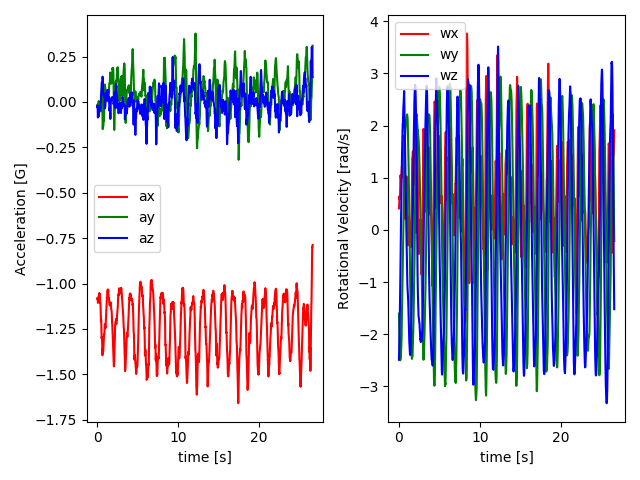
# plot an instance from the data set
# this plot shows 6-axis inertial sensor data recorded by someone doing shoulder pendulum exercise
Xt0 = Xt[0]
f, axes = plt.subplots(nrows=1, ncols=2)
t = np.arange(len(Xt0)) / fs
axes[0].plot(t, Xt0[:, 0], 'r-')
axes[0].plot(t, Xt0[:, 1], 'g-')
axes[0].plot(t, Xt0[:, 2], 'b-')
axes[0].set_xlabel('time [s]')
axes[0].set_ylabel('Acceleration [G]')
axes[0].legend(data['X_labels'][0:3])

axes[1].plot(t, Xt0[:, 3], 'r-')
axes[1].plot(t, Xt0[:, 4], 'g-')
axes[1].plot(t, Xt0[:, 5], 'b-')
axes[1].set_xlabel('time [s]')
axes[1].set_ylabel('Rotational Velocity [rad/s]')
axes[1].legend(data['X_labels'][3:6])

plt.tight_layout()
plt.show()