Resampling Time Series Data

This is a basic example using the pipeline to learn resample a time series

This may be useful for resampling irregularly sampled time series, or for determining an optimal sampling frequency for the data

Out:

/home/david/Code/seglearn/examples/plot_interp.py:44: VisibleDeprecationWarning: Creating an ndarray from ragged nested sequences (which is a list-or-tuple of lists-or-tuples-or ndarrays with different lengths or shapes) is deprecated. If you meant to do this, you must specify 'dtype=object' when creating the ndarray
  X = np.array([np.column_stack([np.arange(len(X[i])) / 50., X[i]]) for i in np.arange(len(X))])
N series in train:  105
N series in test:  35
N segments in train:  1625
N segments in test:  604
Accuracy score:  0.7334437086092715
/home/david/Code/venv3/lib/python3.6/site-packages/seglearn/split.py:100: VisibleDeprecationWarning: Creating an ndarray from ragged nested sequences (which is a list-or-tuple of lists-or-tuples-or ndarrays with different lengths or shapes) is deprecated. If you meant to do this, you must specify 'dtype=object' when creating the ndarray
  Xt_new = np.array(Xt_new)
/home/david/Code/seglearn/examples/plot_interp.py:85: UserWarning: Matplotlib is currently using agg, which is a non-GUI backend, so cannot show the figure.
  plt.show()

# Author: David Burns
# License: BSD

import matplotlib.pyplot as plt
import numpy as np
from sklearn.ensemble import RandomForestClassifier
from sklearn.model_selection import train_test_split, GridSearchCV
from sklearn.preprocessing import StandardScaler

from seglearn.datasets import load_watch
from seglearn.pipe import Pype
from seglearn.split import TemporalKFold
from seglearn.transform import FeatureRep, Segment, Interp


def calc_segment_width(params):
    # number of samples in a 2 second period
    period = params['interp__sample_period']
    return int(2. / period)


# seed RNGESUS
np.random.seed(123124)

# load the data
data = load_watch()

X = data['X']
y = data['y']

# I am adding in a column to represent time (50 Hz sampling), since my data doesn't include it
# the Interp class assumes time is the first column in the series
X = np.array([np.column_stack([np.arange(len(X[i])) / 50., X[i]]) for i in np.arange(len(X))])

clf = Pype([('interp', Interp(1. / 25., categorical_target=True)),
            ('segment', Segment(width=100)),
            ('features', FeatureRep()),
            ('scaler', StandardScaler()),
            ('rf', RandomForestClassifier(n_estimators=20))])

# split the data
X_train, X_test, y_train, y_test = train_test_split(X, y, test_size=0.25)

clf.fit(X_train, y_train)
score = clf.score(X_test, y_test)

print("N series in train: ", len(X_train))
print("N series in test: ", len(X_test))
print("N segments in train: ", clf.N_train)
print("N segments in test: ", clf.N_test)
print("Accuracy score: ", score)

# lets try a few different sampling periods
# temporal splitting of data
splitter = TemporalKFold(n_splits=3)
Xs, ys, cv = splitter.split(X, y)

# here we use a callable parameter to force the segmenter width to equal 2 seconds
# note this is an extension of the sklearn api for setting class parameters
par_grid = {'interp__sample_period': [1. / 5., 1. / 10., 1. / 25., 1. / 50.],
            'segment__width': [calc_segment_width]}

clf = GridSearchCV(clf, par_grid, cv=cv)
clf.fit(Xs, ys)
scores = clf.cv_results_['mean_test_score']
stds = clf.cv_results_['std_test_score']

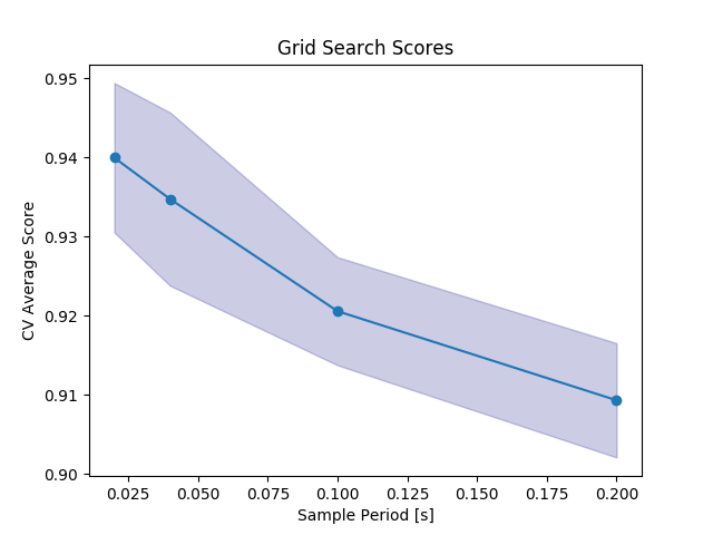
plt.plot(par_grid['interp__sample_period'], scores, '-o')
plt.title("Grid Search Scores")
plt.xlabel("Sample Period [s]")
plt.ylabel("CV Average Score")
plt.fill_between(par_grid['interp__sample_period'], scores - stds, scores + stds, alpha=0.2,
                 color='navy')
plt.show()