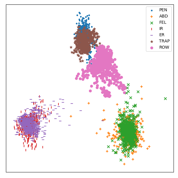
Linear Discriminant Analysis

This example demonstrates how the pipeline can be used to perform transformation of time series data, such as linear discriminant analysis for visualization purposes

Out:

/home/david/Code/seglearn/examples/plot_lda.py:51: UserWarning: Matplotlib is currently using agg, which is a non-GUI backend, so cannot show the figure.
  plt.show()

# Author: David Burns
# License: BSD

import matplotlib.pyplot as plt
import numpy as np
from sklearn.discriminant_analysis import LinearDiscriminantAnalysis

import seglearn as sgl


def plot_embedding(emb, y, y_labels):
    # plot a 2D feature map embedding
    x_min, x_max = np.min(emb, 0), np.max(emb, 0)
    emb = (emb - x_min) / (x_max - x_min)

    NC = len(y_labels)
    markers = ['.', '+', 'x', '|', '_', '*', 'o']

    fig = plt.figure()
    fig.set_size_inches(6, 6)

    for c in range(NC):
        i = y == c
        plt.scatter(emb[i, 0], emb[i, 1], marker=markers[c], label=y_labels[c])

    plt.xticks([]), plt.yticks([])
    plt.legend()
    plt.tight_layout()


# load the data
data = sgl.load_watch()
X = data['X']
y = data['y']

# create a pipeline for LDA transformation of the feature representation
clf = sgl.Pype([('segment', sgl.Segment()),
                ('ftr', sgl.FeatureRep()),
                ('lda', LinearDiscriminantAnalysis(n_components=2))])

X2, y2 = clf.fit_transform(X, y)
plot_embedding(X2, y2.astype(int), data['y_labels'])
plt.show()